Parsing Apache logs is a well documented Hive use case, but when I tried to implement it recently using RegexSerDe I could not get it to work. I copied the gzipped Apache logs to S3 and used Amazon Elastic MapReduce to create the Hive table as documented, but when I tried to select from the table all of the values came out as NULL. I tried some different versions of the Hive DDL that I found online, but none of them worked.

Rather than continuing to debug that implementation I decided to take a different approach. Rather than using RegexSerDe, I just created a table with one column representing the entire log line and used the Hive regexp_extract function to select various virtual columns.

For example, here’s the table in Hive:

1
2
3
4
5
6

CREATE EXTERNAL TABLE IF NOT EXISTS apache_log (
  log_line STRING
)
PARTITIONED BY (dt STRING)
STORED AS TEXTFILE
LOCATION '${BUCKET}/apache';

And here’s a query to extract the HTTP response code from each log line so we can count how many times each response code occurs in a given day:

1
2
3
4
5

select regexp_extract(log_line,' ([0-9]{3}) (?:.*[0-9]{1,6})',1) as http_response_code, 
  count(1)
from apache_log 
where dt='2013-08-12'
group by regexp_extract(log_line,' ([0-9]{3}) (?:.*[0-9]{1,6})',1);

The rest of my project mostly involved parsing the request. I was going to have to use regexp_extract to do that anyways, so using that function to do all of the parsing was pretty easy.

A Brief History of Redis at Flite

Here at Flite we use Redis as the backend for realtime metrics and the ad debugger. We use counters to tabulate various events such as impressions, interactions, and content events; as well as storing the body of each event - about 30 counters per event. Until recently, this data lived on a single Redis server for about 4 hours before it expired or was replaced by newer data. Over the past year of using this setup we have experienced problems with our data set growing too large and pushing data out in as little as 2 hours. We solved these early growing pains by moving to a server with more memory and code optimizations such as gzipping.

However a single server cannot scale forever…

Recently I started a project that required deleting millions of rows of data from various MySQL tables. Many of the queries which identifed the rows to delete required several joins. I decided to use common_schema’s split() function to break the deletes into chunks, but when I started running the queries in common_schema some of them failed to delete any data. I assume the failures were related to the complexity of the multi-table delete statements.

Thiking of this as a two step problem a natural workaround emerged. The two steps are:

1. Identify the rows to delete
2. Delete the rows

I want to use split() for step 2, but I don’t really need it for step 1.

I decided to create a new table to store the ids which define the rows to delete, then populate that table, and use a simpler multi-table delete statement to execute the deletes using split(). So far this workaround has allowed me to execute several separate delete statements, each deleting millions of rows in chunks.

Here’s an example. Say I want to execute a delete like this:

1
2
3
4
5
6
7

delete ad_tag.*
from ad_tag
  inner join ad on ad.id = ad_tag.ad_id
  inner join user_account on user_account.id = ad.user_id
  inner join organization on organization.id = ad.org_id
where user_account.service_level = 0
  or organization.service_level = 0;

I can delete the same rows using the two step approach discussed above as follows:

1
2
3
4
5
6
7
8
9
10
11
12
13
14
15
16
17
18
19
20
21
22
23
24

create table if not exists temp_rows_to_delete (
  ad_id int not null,
  primary key (ad_id)
) Engine=InnoDB;

insert ignore into temp_rows_to_delete (ad_id)
select ad.id
from ad
  inner join user_account on user_account.id = ad.user_id
  inner join organization on organization.id = ad.org_id
where user_account.service_level = 0
  or organization.service_level = 0;

set @script := "
  split(temp_rows_to_delete: delete ad_tag.*
from temp_rows_to_delete
inner join ad_tag on ad_tag.ad_id = temp_rows_to_delete.ad_id
  )
  SELECT $split_total_rowcount AS 'rows deleted so far';
";

call common_schema.run(@script);

drop table if exists temp_rows_to_delete;

There are several approaches to count the occurrences of a substring inside a larger string in MySQL. Some people use replace() and length() (I would use char_length() instead) to do it. Others use stored functions. Recently I had to count the occurrences of a certain key across many rows of JSON. Instead of writing my own query using one of the approaches mentioned above I decided to use common_schema.

In the past I’ve discussed JSON parsing in MySQL using common_schema. In this case I didn’t need to parse the JSON, just to count keys, so I used the get_num_tokens() function instead. That function is designed to count the number of tokens in delimited text. It does so essentially by counting the number of delimiters and then adding one. Since I’m looking for a certain key and treating that key as the delimiter, I just need to subtract one from the result of get_num_tokens() to get the key/delimtier count instead of the token count.

Here’s an example:

1
2
3
4
5
6
7

mysql> set @haystack := '{"needles":["needle":{"type":"sewing","is_sharp":"yes"},"needle":{"type":"knitting","is_sharp":"no"},"needle":{"type":"acupunture","is_sharp":"yes"}]}';
Query OK, 0 rows affected (0.00 sec)

mysql> select @haystack, common_schema.get_num_tokens(@haystack, '"needle"')-1 as needles\G
*************************** 1. row ***************************
@haystack: {"needles":["needle":{"type":"sewing","is_sharp":"yes"},"needle":{"type":"knitting","is_sharp":"no"},"needle":{"type":"acupunture","is_sharp":"yes"}]}
  needles: 3

As documented in the MySQL Reference Manual:

a UNIQUE index permits multiple NULL values for columns that can contain NULL.

There are many scenarios in which this behavior is desirable. For example imagine you create a user table and require an email address, but you want username to be optional. You make the username column nullable, but you also want to make sure all non-null values in the column are unique, so it makes sense to add a UNIQUE INDEX. If the UNIQUE INDEX didn’t allow multiple NULL values then you would need to move the username column to a separate table in order to both maintain uniqueness and allow users without usernames.

But there are also plenty of scenarios where this behavior can cause problems. For example, consider aggregated fact tables in a star schema. You typically only want one row for a given combination of dimension values, and you can enforce this using a UNIQUE INDEX. However, if one or more of the dimension columns are nullable then you are at risk of having duplicate data.

Recently this affected an ETL process at Flite that loads data into a MySQL star schema. Sometimes I need to re-run all or part of the ETL process based on failures, and I rely on unique indexes to prevent the same data from being loaded into the star schema more than once. Most of my dimension columns do not allow null values, but a few of them do, which led to some data duplication when I re-ran pieces of the ETL flow. To fix the problem I identified all of the affected columns, cleaned up the existing data, made the columns NOT NULL, and came up with other values to use for missing data: For text columns I replaced NULL with the empty string ''. For numeric values I replaced NULL with 0.

Read on for details on how to find and fix this problem. For my examples I will use the Foodmart sample database from Pentaho.

Metadata Is Just Data

Computers are their own meta. Alan Turing, with inspiration from Kurt Gödel and his Incompleteness Theorem, remarkably before computers were even invented. Alonzo Church showed pretty much the same thing, at about the same time, so the result of their work is often called the Church-Turing theorem. The goals of these 20th-century intellectual giants were epistemological in nature, and the implications are profound. It seems surprising, then, when applied needs not only take advantage of these implications, but in so doing, also use some of the same techniques pioneered in these philosophical quests. This is the story of how, in a small way, Flite piggybacks on the shoulders of these giants.

Flite’s mission is to empower advertisers. To do this we need a metasystem - a system to interpret the metadata of display advertisements and set up the appropriate environment in which to run the ad. The result is called the Flite Ad Runtime (the “runtime”), and the implications, while far less profound than those of the work of Gödel, Church and Turing, are nonetheless good news for people with a need to create and distribute rich, interactive advertising. I inherited the task of maintaining and extending the runtime, and have been delighted to find that it contains many of the same techniques used by Gödel/Church/Turing (GCT) in their firmament-busting proofs.

There are a several aspects of GCT in the runtime that I would like to describe, but I will start with only one, in the hope that some other sentient beings are likewise afflicted with an obsession about this stuff, and demand for more will be at least measurable (measurable in the sense that we can measure when someone spends more than 2 minutes reading this post). I sum up today’s theme thusly: Metadata is just data.

Kurt Gödel, Time Magazine’s Mathematician of the Century, has been called a “metamathematician,” someone that works with mathematical systems. In his Weltanschauung-shattering Incompleteness Theorem, he actually shows that any really cool system of mathematics (a “formal system”) can be repurposed to become its own metasystem - that is, it can be used to talk about itself, to reveal truths about the system itself, not just truths within the system. This is quite remarkable, so I will repeat it: To study the system of mathematics, all we need is mathematics itself.

A while back one of my foreign keys started causing trouble. The problem was that some parent rows had tens of thousand of child rows, and the foreign key was defined with CASCADE DELETE enabled. When we deleted one of those parent rows on a master database, it took several seconds to execute the delete because of the cascade. This led to latency for the end user, and also led to replication delays.

The immediate solution was make the application tolerant of orphaned rows in the child table and to drop the explicit foreign key constraint.

I didn’t really want to leave those orphaned rows hanging around in the child table, so I decided to implement an asynchronous process to delete the orphaned rows on a scheduled basis. Read on for a description of that process.

After learning the secret ingredient for Flite’s Q2 hackday was big data, we spent a lot of time looking at the many public data sets available, and deciding what to incorporate in our project. One notable departure from the typical hackday format for Q2 was that we were not required to develop something specifically for the Flite platform.

This interested us, and looking at the plethora of public data sets available on the web, we kept coming back to the sets that hit closest to home: San Francisco City data.

The San Francisco Open Data Portal provides a wide range of data sets containing information related to campaign finance contribution, public transportation (MUNI), and even listings of locations for movies shot in the city.

Being somewhat typical, modern city dwellers, one thing we love about San Francisco is the many purveyors of, and availability for, tasty food and beverage. Given this preoccupation with eats, drinks, etc., one of the most interesting data sets available to us was the Health Department’s repository of Restaurant Health Inspection Scores.

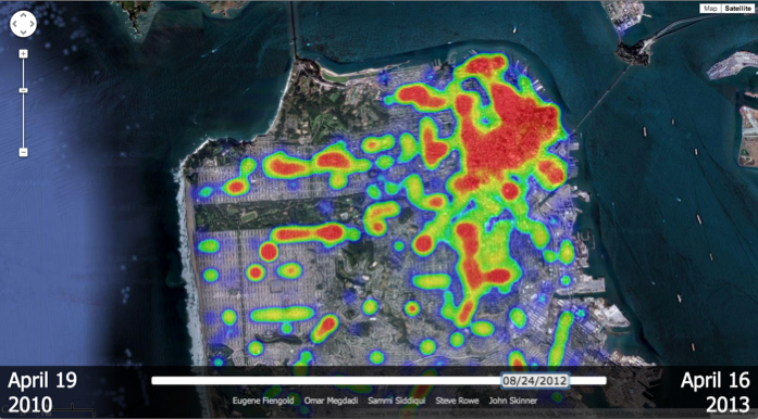
We set out to build a visualization of these scores by plotting this data in an application using Google Maps.

Red sections indicate lower (high risk) health scores. Blue sections represent higher (low risk) health scores.

Our hope was to provide a heat map of the city indicating areas that have more dubious or more positive health scores. Ultimately the visualization provides more of a heat map of restaurants inspected over a period of time. Looking at the results, we came to the conclusion that health score filtering options would be necessary to accomplish what we were after.

For a fully functional visualization of health scores on a map, visit sfscores.com.

Bon Appétit!

Team Asparagus (Steve Rowe, Saami Siddiqui, Omar Megdadi, Eugene Feingold, John Skinner)

During Flite’s Q2 hackday, the secret ingredient was “Big data sets” and every group could work on any hack that deals with the secret ingredient. During the brainstorming process, our group “Beets” thought of utilizing the large amount of data generated from our ad metrics system when a user interacts with an ad.

When a user interacts with a Flite ad, we collect all actions made by the user within the ad. The common interactions we collect include clicks, scrolls, hovers, clickthroughs and many more. Each interaction contains a series of information, including the sequence number, the spot where the interaction happened (x,y position relative to the ad), component name, etc. With this information we can reconstruct the whole user session.

As we have this huge amount of interaction data, we thought of building a feature which shows the most common user path for a specific ad. This can help data analysts see how our current users are interacting with the ad, when they are leaving the ad, and find patterns to improve the interaction rate.

For any given ad:

1. Grab all interaction data, grouped by session.
2. For each session, remove interactions that are not important like hovers, rollovers, rollouts etc., and generate new sequence numbers.
3. Group all sessions by its sequence number and component name.

Have you ever wondered who clicks on digital ads? Is it people who live in the most tech savvy, modern cities? Is it someone with too much time on their hands in a remote corner of North Dakota? Do idle hands lead to higher interactions in ads? Team Garlic wanted to know and their Hack Day goal was to find to out more about who clicks on Flite ads by using our own data combined with open data on census.gov.

The plan was to gather the smallest, but most relevant data set as quickly as possible, see what it told us, and show it off. Ike and Angel mined our own data in Hive for the top impressions, interactions, and browser by city and state. Meanwhile, Andy and Matt decided to see what kind census data we could get from census.gov regarding population, income, gender, and employment rate. Once we had all of that info, Ike was going to merge the data in MySQL, Angel would then analyze it for trends, and Andy would build a page to display the data.

Before we went out and started gathering data, we decided to form a hypothesis about correlations between census data and Flite usage data. The best idea we could come up with based on state-level data was that a higher unemployment rate may correlate with a higher time on unit, engagement rate, and/or interaction rate. Read on to find out if our hypothesis was valid.